OpenAnnotate sheds light on single-cell data analyses
Bulk openness score of peaks in the target single-cell chromatin accessibility sequencing (scCAS) data (e.g. scATAC-seq data) can be adopted as a reference to facilitate the analysis of scCAS data.
This reference-based idea has been successfully applied to the characterization (Cell 2018, Nature Communications 2021) and imputation (Genome Biology 2020) of scCAS data.
In this notebook, we introduce a straightforward approach to incorporate the openness data annotated by OpenAnnotate as a reference to characterize scCAS data:
- 1) Perform the term frequency-inverse document frequency (TF-IDF) transformation to normalize the scCAS data matrix;
- 2) Annotate the bulk openness of peaks in the scCAS data by OpenAnnotate (referred as the reference data);
- 3) Apply PCA on the reference data and use the learned projection vectors to project TF-IDF transformed scCAS data.
We first demonstrate the effectiveness of this reference projection approach using a scATAC-seq dataset of human hematopoietic cells (referred as the Buenrostro2018 dataset), as a recent benchmark study (Genome Biology 2019).
We then show the performance of this reference projection approach on other three scCAS datasets: the GMvsHEK (Science 2015), GMvsHL (Science 2015), and InSilico (Nature 2015) datasets.
We note that this reference projection approach implicitly assumes that all the biological variation is shared in single-cell and the reference data, as it only uses the projection vectors learned from the reference bulk data and do not use single-cell data to learn the projection vectors, even though it can further benefit the characterization of scCAS data.
import sklearn
import pandas as pd
import numpy as np
As the recent benchmark study (Genome Biology 2019), we evaluate the performance of the reference projection approach by data visualization and cell clustering.
To be more specific, we first obtain the low-dimensional representation (first 30 PCs). We then implement UMAP visualization using Scanpy, a widely-used Python library for the analysis of single-cell data, with default settings, and perform cell clustering (hierarchical clustering, k-means, and Louvain clustering) using the source code obtained from the benchmark study (Genome Biology 2019).
# Define the functions for evaluation
import scanpy as sc
from sklearn.cluster import KMeans
from sklearn.cluster import AgglomerativeClustering
from sklearn.metrics.cluster import adjusted_rand_score
from sklearn.metrics.cluster import adjusted_mutual_info_score
from sklearn.metrics.cluster import homogeneity_score

def run_hc(adata,n_cluster):
    hc = AgglomerativeClustering(n_clusters=n_cluster).fit(adata.X)
    adata.obs['hc'] = pd.Series(hc.labels_,index=adata.obs.index).astype('category')
    ari = adjusted_rand_score(adata.obs['label'], adata.obs['hc'])
    ami = adjusted_mutual_info_score(adata.obs['label'], adata.obs['hc'])
    homo = homogeneity_score(adata.obs['label'], adata.obs['hc'])
    print('HC:\t\tARI: %.3f, AMI: %.3f, Homo: %.3f' % (ari,ami,homo))
    return (adata.obs['label'], adata.obs['hc'], ari,ami,homo)

def run_kmeans(adata,n_cluster):
    kmeans = KMeans(n_clusters=n_cluster, random_state=2019).fit(adata.X)
    adata.obs['kmeans'] = pd.Series(kmeans.labels_,index=adata.obs.index).astype('category')
    ari = adjusted_rand_score(adata.obs['label'], adata.obs['kmeans'])
    ami = adjusted_mutual_info_score(adata.obs['label'], adata.obs['kmeans'])
    homo = homogeneity_score(adata.obs['label'], adata.obs['kmeans'])
    print('kmeans:\t\tARI: %.3f, AMI: %.3f, Homo: %.3f' % (ari,ami,homo))
    return (adata.obs['label'], adata.obs['kmeans'], ari,ami,homo)

def run_louvain(adata,n_cluster,range_min=0,range_max=3,max_steps=30):
    this_step = 0
    this_min = float(range_min)
    this_max = float(range_max)
    while this_step < max_steps:
#         print('step ' + str(this_step))
        this_resolution = this_min + ((this_max-this_min)/2)
        sc.tl.louvain(adata,resolution=this_resolution)
        this_clusters = adata.obs['louvain'].nunique()
#         print('got ' + str(this_clusters) + ' at resolution ' + str(this_resolution))
        if this_clusters > n_cluster:
            this_max = this_resolution
        elif this_clusters < n_cluster:
            this_min = this_resolution
        else:
#             return(this_resolution, adata)
            ari = adjusted_rand_score(adata.obs['label'], adata.obs['louvain'])
            ami = adjusted_mutual_info_score(adata.obs['label'], adata.obs['louvain'])
            homo = homogeneity_score(adata.obs['label'], adata.obs['louvain'])
            print('Louvain:\tARI: %.3f, AMI: %.3f, Homo: %.3f' % (ari,ami,homo))
            return (adata.obs['label'], adata.obs['louvain'], ari,ami,homo)
        this_step += 1
    print('Cannot find the number of clusters')
#     print('Clustering solution from last iteration is used:' + str(this_clusters) + ' at resolution ' + str(this_resolution))
    ari = adjusted_rand_score(adata.obs['label'], adata.obs['louvain'])
    ami = adjusted_mutual_info_score(adata.obs['label'], adata.obs['louvain'])
    homo = homogeneity_score(adata.obs['label'], adata.obs['louvain'])
    print('Louvain:\t\tARI: %.3f, AMI: %.3f, Homo: %.3f' % (ari,ami,homo))
    return (adata.obs['label'], adata.obs['louvain'], ari,ami,homo)

def evaluate(sc_tfidf_fm, sc_labels):
    adata = sc.AnnData(sc_tfidf_fm)
    adata.obs['label'] = sc_labels
    sc.pp.neighbors(adata, use_rep='X')
    sc.tl.umap(adata)
    sc.pl.umap(adata, color=['label'])

    n_cluster = np.unique(sc_labels).shape[0]
    _ = run_hc(adata, n_cluster)
    _ = run_kmeans(adata, n_cluster)
    _ = run_louvain(adata, n_cluster)
!mkdir output
The Buenrostro2018 dataset
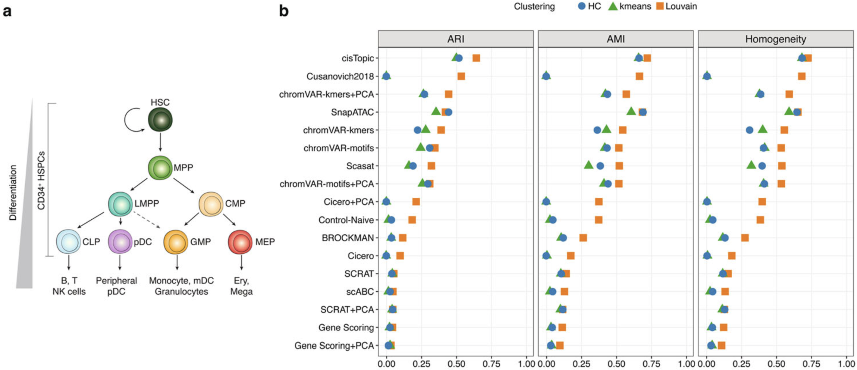
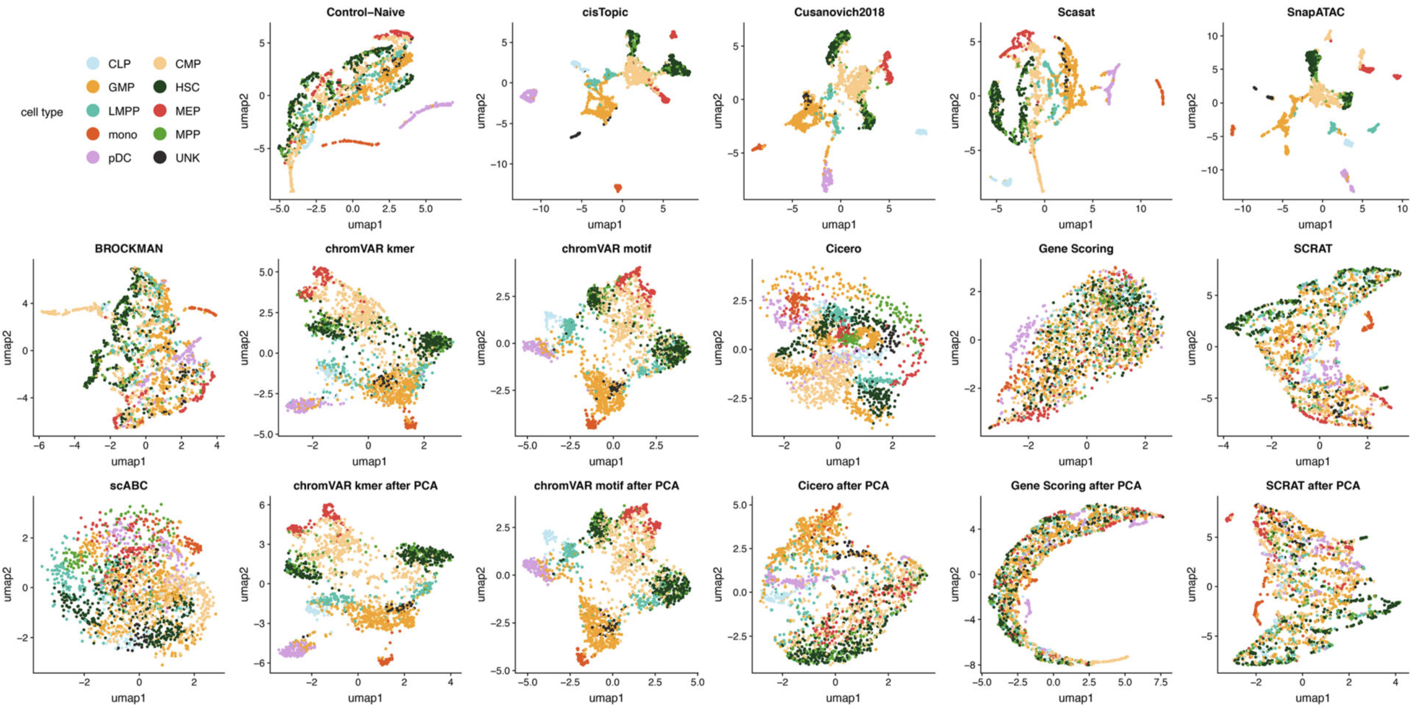
We collected the benchmarking results provided by Chen et al. (Genome Biology 2019).
a Developmental roadmap of cell types analyzed.
b Dot plot of scores for each metric to quantitatively measure the clustering performance of each method, sorted by maximum ARI score.

UMAP visualization of the feature matrix produced by each method for the Buenrostro2018 dataset.

The raw data of Buenrostro2018 dataset is available at Supplementary and GEO.
For convenience, we provide the data preprocessed according to the source Matlab codes of original study. The data can be downloaded here.
# Load data
import pickle
with open('./data/Buenrostro2018.pkl', 'rb') as f:
    obj = pickle.load(f)
obj.keys()
sc_counts = obj['sc_counts']
sc_peaks  = obj['sc_peaks']
sc_labels = obj['sc_labels']
print(sc_counts.shape, len(sc_peaks), len(sc_labels))
sc_peaks[:3]
pd.value_counts(sc_labels)
Generate the BED file containing single-cell peaks to be submitted to OpenAnnotate.
fout = open('./output/Buenrostro2018.bed','w')
for i in sc_peaks:
    chrom, start, end = i.split('_')
    fout.write("%s\t%s\t%s\t.\t.\t.\n"%(chrom, start, end))
fout.close()
Now we can submit the BED file to OpenAnnotate on the 'Annotate' page:
Upload the file, choose 'DNase-seq' (ENCODE) and 'Homo sapiens (GRCh37/hg19)', specify the cell type of 'All biosample types', enable the option of 'Region-based annotation', and submit the task.
Download the annotation results by the links sent to mailbox or the online Download button.
Here we take raw read openness (readopen.txt.gz) and narrow peak openness (peakopen.txt.gz) as examples.
# In this demo, you can directly use the following Download links for convenience.
!wget http://health.tsinghua.edu.cn/openness/anno/task/2020/1205/14031434/anno/readopen.txt.gz -O ./output/Buenrostro2018.readopen.txt.gz
!wget http://health.tsinghua.edu.cn/openness/anno/task/2020/1205/14031434/anno/peakopen.txt.gz -O ./output/Buenrostro2018.peakopen.txt.gz
Uncompress the files and load the results using Numpy. The first four columns consist of chromosomes, starting sites, terminating sites and strands, respectively. The remaining columns corresponds to different DNase-seq experiments. The details of these experiments can be accessed from the Head file (e.g., http://health.tsinghua.edu.cn/openness/anno/task/2020/1205/14031434/anno/head.txt.gz).
!gunzip ./output/*.txt.gz
readopen = np.loadtxt('./output/Buenrostro2018.readopen.txt',dtype=str)
readopen = readopen[:,4:].astype(float)
readopen.shape
# Filter out zero cells and peaks in scCAS data
select_cell = np.sum(sc_counts,axis=0) != 0
select_peak = np.sum(sc_counts,axis=1) != 0

sc_counts = sc_counts[:, select_cell]
sc_labels = np.array(sc_labels)[select_cell]

sc_counts = sc_counts[select_peak, :]
readopens = readopen[select_peak, :]
print(sc_counts.shape, readopens.shape)
# Perform TF-IDF
nfreqs = 1.0 * sc_counts / np.tile(np.sum(sc_counts,axis=0), (sc_counts.shape[0],1))
sc_tfidf  = nfreqs * np.tile(np.log(1 + 1.0 * sc_counts.shape[1] / np.sum(sc_counts,axis=1)).reshape(-1,1), (1,sc_counts.shape[1]))
# Apply PCA on the reference data, and use the learned projection vectors to project TF-IDF transformed scCAS data
from sklearn.decomposition import PCA
ref_pca = PCA(svd_solver='full', random_state=0).fit(readopens.T)
sc_tfidf_refProj = ref_pca.transform(sc_tfidf.T)
print(sc_tfidf_refProj.shape)
# Evaluate the performance
evaluate(sc_tfidf_refProj[:,:30], sc_labels)
The alternative approach, which constructs the reference using peak openness, also achieves similar performance:
peakopen = np.loadtxt('./output/Buenrostro2018.peakopen.txt',dtype=str)
peakopen = peakopen[:,4:].astype(float)
peakopens = peakopen[select_peak, :]
print(sc_counts.shape, peakopens.shape)
from sklearn.decomposition import PCA
ref_pca = PCA(svd_solver='full', random_state=0).fit(peakopens.T)
sc_tfidf_refProj = ref_pca.transform(sc_tfidf.T)
print(sc_tfidf_refProj.shape)
evaluate(sc_tfidf_refProj[:,:30], sc_labels)
As the data visualization shown above, the straightforward reference projection approach successfully distinguished most of the hematopoietic cells. The visualization result is comparable to state-of-the-art methods in the benchmark study (Genome Biology 2019).
For the cell clustering, the reference projection approach achieves overall top-three performance, which again indicates the effectiveness of this straightforward approach.
The GMvsHEK dataset
We then show the performance of this reference projection approach on the GMvsHEK (Science 2015) dataset.
For convenience, we provide the data preprocessed according to the original study. The data can be downloaded here.
import pickle
with open('./data/GMvsHEK.pkl', 'rb') as f:
    obj = pickle.load(f)
obj.keys()
sc_counts = obj['sc_counts']
sc_peaks  = obj['sc_peaks']
sc_labels = obj['sc_labels']
print(sc_counts.shape, len(sc_peaks), len(sc_labels))
sc_peaks[:3]
pd.value_counts(sc_labels)
Generate BED file containing single-cell peaks to be submitted to OpenAnnotate.
fout = open('./output/GMvsHEK.bed','w')
for i in sc_peaks:
    chrom, start, end = i.split('_')
    fout.write("%s\t%s\t%s\t.\t.\t.\n"%(chrom, start, end))
fout.close()
Now we can submit the BED file to OpenAnnotate on the 'Annotate' page:
Upload the file, choose 'DNase-seq' (ENCODE) and 'Homo sapiens (GRCh37/hg19)', specify the cell type of 'All biosample types', enable the option of 'Region-based annotation', and submit the task.
!wget http://health.tsinghua.edu.cn/openness/anno/task/2020/1205/15091699/anno/readopen.txt.gz -O ./output/GMvsHEK.readopen.txt.gz
!wget http://health.tsinghua.edu.cn/openness/anno/task/2020/1205/15091699/anno/peakopen.txt.gz -O ./output/GMvsHEK.peakopen.txt.gz
!gunzip ./output/*.txt.gz
readopen = np.loadtxt('./output/GMvsHEK.readopen.txt',dtype=str)
readopen = readopen[:,4:].astype(float)
readopen.shape
select_cell = np.sum(sc_counts,axis=0) != 0
select_peak = np.sum(sc_counts,axis=1) != 0

sc_counts = sc_counts[:, select_cell]
sc_labels = np.array(sc_labels)[select_cell]

sc_counts = sc_counts[select_peak, :]
readopens = readopen[select_peak, :]
print(sc_counts.shape, readopens.shape)
nfreqs = 1.0 * sc_counts / np.tile(np.sum(sc_counts,axis=0), (sc_counts.shape[0],1))
sc_tfidf  = nfreqs * np.tile(np.log(1 + 1.0 * sc_counts.shape[1] / np.sum(sc_counts,axis=1)).reshape(-1,1), (1,sc_counts.shape[1]))
from sklearn.decomposition import PCA
ref_pca = PCA(svd_solver='full', random_state=0).fit(readopens.T)
sc_tfidf_refProj = ref_pca.transform(sc_tfidf.T)
print(sc_tfidf_refProj.shape)
evaluate(sc_tfidf_refProj[:,:30], sc_labels)
peakopen = np.loadtxt('./output/GMvsHEK.peakopen.txt',dtype=str)
peakopen = peakopen[:,4:].astype(float)
peakopens = peakopen[select_peak, :]
print(sc_counts.shape, peakopens.shape)
from sklearn.decomposition import PCA
ref_pca = PCA(svd_solver='full', random_state=0).fit(peakopens.T)
sc_tfidf_refProj = ref_pca.transform(sc_tfidf.T)
print(sc_tfidf_refProj.shape)
evaluate(sc_tfidf_refProj[:,:30], sc_labels)
The GMvsHL dataset
We then show the performance of this reference projection approach on the GMvsHL (Science 2015) dataset.
For convenience, we provide the data preprocessed according to the original study. The data can be downloaded here.
import pickle
with open('./data/GMvsHL.pkl', 'rb') as f:
    obj = pickle.load(f)
obj.keys()
sc_counts = obj['sc_counts']
sc_peaks  = obj['sc_peaks']
sc_labels = obj['sc_labels']
print(sc_counts.shape, len(sc_peaks), len(sc_labels))
sc_peaks[:3]
pd.value_counts(sc_labels)
Generate BED file containing single-cell peaks to be submitted to OpenAnnotate.
fout = open('./output/GMvsHL.bed','w')
for i in sc_peaks:
    chrom, start, end = i.split('_')
    fout.write("%s\t%s\t%s\t.\t.\t.\n"%(chrom, start, end))
fout.close()
Now we can submit the BED file to OpenAnnotate on the 'Annotate' page:
Upload the file, choose 'DNase-seq' (ENCODE) and 'Homo sapiens (GRCh37/hg19)', specify the cell type of 'All biosample types', enable the option of 'Region-based annotation', and submit the task.
!wget http://health.tsinghua.edu.cn/openness/anno/task/2020/1205/15085351/anno/readopen.txt.gz -O ./output/GMvsHL.readopen.txt.gz
!wget http://health.tsinghua.edu.cn/openness/anno/task/2020/1205/15085351/anno/peakopen.txt.gz -O ./output/GMvsHL.peakopen.txt.gz
!gunzip ./output/*.txt.gz
readopen = np.loadtxt('./output/GMvsHL.readopen.txt',dtype=str)
readopen = readopen[:,4:].astype(float)
readopen.shape
select_cell = np.sum(sc_counts,axis=0) != 0
select_peak = np.sum(sc_counts,axis=1) != 0

sc_counts = sc_counts[:, select_cell]
sc_labels = np.array(sc_labels)[select_cell]

sc_counts = sc_counts[select_peak, :]
readopens = readopen[select_peak, :]
print(sc_counts.shape, readopens.shape)
nfreqs = 1.0 * sc_counts / np.tile(np.sum(sc_counts,axis=0), (sc_counts.shape[0],1))
sc_tfidf  = nfreqs * np.tile(np.log(1 + 1.0 * sc_counts.shape[1] / np.sum(sc_counts,axis=1)).reshape(-1,1), (1,sc_counts.shape[1]))
from sklearn.decomposition import PCA
ref_pca = PCA(svd_solver='full', random_state=0).fit(readopens.T)
sc_tfidf_refProj = ref_pca.transform(sc_tfidf.T)
print(sc_tfidf_refProj.shape)
evaluate(sc_tfidf_refProj[:,:30], sc_labels)
peakopen = np.loadtxt('./output/GMvsHL.peakopen.txt',dtype=str)
peakopen = peakopen[:,4:].astype(float)
peakopens = peakopen[select_peak, :]
print(sc_counts.shape, peakopens.shape)
from sklearn.decomposition import PCA
ref_pca = PCA(svd_solver='full', random_state=0).fit(peakopens.T)
sc_tfidf_refProj = ref_pca.transform(sc_tfidf.T)
print(sc_tfidf_refProj.shape)
evaluate(sc_tfidf_refProj[:,:30], sc_labels)
The InSilico dataset
We then show the performance of this reference projection approach on the InSilico (Nature 2015) dataset.
For convenience, we provide the data preprocessed according to the original study. The data can be downloaded here.
import pickle
with open('./data/InSilico.pkl', 'rb') as f:
    obj = pickle.load(f)
obj.keys()
sc_counts = obj['sc_counts']
sc_peaks  = obj['sc_peaks']
sc_labels = obj['sc_labels']
print(sc_counts.shape, len(sc_peaks), len(sc_labels))
sc_peaks[:3]
pd.value_counts(sc_labels)
Generate BED file containing single-cell peaks to be submitted to OpenAnnotate.
fout = open('./output/InSilico.bed','w')
for i in sc_peaks:
    chrom, start, end = i.split('_')
    fout.write("%s\t%s\t%s\t.\t.\t.\n"%(chrom, start, end))
fout.close()
Now we can submit the BED file to OpenAnnotate on the 'Annotate' page:
Upload the file, choose 'DNase-seq' (ENCODE) and 'Homo sapiens (GRCh37/hg19)', specify the cell type of 'All biosample types', enable the option of 'Region-based annotation', and submit the task.
!wget http://health.tsinghua.edu.cn/openness/anno/task/2020/1205/15082882/anno/readopen.txt.gz -O ./output/InSilico.readopen.txt.gz
!wget http://health.tsinghua.edu.cn/openness/anno/task/2020/1205/15082882/anno/peakopen.txt.gz -O ./output/InSilico.peakopen.txt.gz
!gunzip ./output/*.txt.gz
readopen = np.loadtxt('./output/InSilico.readopen.txt',dtype=str)
readopen = readopen[:,4:].astype(float)
readopen.shape
select_cell = np.sum(sc_counts,axis=0) != 0
select_peak = np.sum(sc_counts,axis=1) != 0

sc_counts = sc_counts[:, select_cell]
sc_labels = np.array(sc_labels)[select_cell]

sc_counts = sc_counts[select_peak, :]
readopens = readopen[select_peak, :]
print(sc_counts.shape, readopens.shape)
nfreqs = 1.0 * sc_counts / np.tile(np.sum(sc_counts,axis=0), (sc_counts.shape[0],1))
sc_tfidf  = nfreqs * np.tile(np.log(1 + 1.0 * sc_counts.shape[1] / np.sum(sc_counts,axis=1)).reshape(-1,1), (1,sc_counts.shape[1]))
from sklearn.decomposition import PCA
ref_pca = PCA(svd_solver='full', random_state=0).fit(readopens.T)
sc_tfidf_refProj = ref_pca.transform(sc_tfidf.T)
print(sc_tfidf_refProj.shape)
evaluate(sc_tfidf_refProj[:,:30], sc_labels)
peakopen = np.loadtxt('./output/InSilico.peakopen.txt',dtype=str)
peakopen = peakopen[:,4:].astype(float)
peakopens = peakopen[select_peak, :]
print(sc_counts.shape, peakopens.shape)
from sklearn.decomposition import PCA
ref_pca = PCA(svd_solver='full', random_state=0).fit(peakopens.T)
sc_tfidf_refProj = ref_pca.transform(sc_tfidf.T)
print(sc_tfidf_refProj.shape)
evaluate(sc_tfidf_refProj[:,:30], sc_labels)
The data visualization and cell clustering performance on the GMvsHEK, GMvsHL and InSilico datasets further shows that OpenAnnotate can shed light on single-cell data analyses.
We note that peak openness usually has lower noise than read openness because it is based on peaks (regions in a genome) that have been enriched with aligned reads. Therefore, the reference constructed from peak openness is preferred than that constructed from read openness, especially when there are massive peaks/regions/features in the scCAS data (e.g., the Buenrostro2018 dataset).
Besides, since the reference projection approach implicitly assumes that all the biological variation is shared in single-cell and reference data, statistical or machine learning methods can be developed to better characterize the scCAS data by, for example, simultaneously modeling 1) the shared biological variation among scCAS data and reference data, and 2) the unique biological variation in scCAS data that identifies novel cell subpopulations.
To summarize, the above results demonstrate the potential that one can incorporate openness scores annotated by OpenAnnotate as a reference to facilitate the analyses of scCAS data.